Es un Índice, simplemente tienes que hacer Click en el Posts que sea de tu interés y directamente entrarás en el contenido.
2. Clasificación de los Ultrasonidos.
3. La Onda Ultrasónica. Características.
4. Magnitudes de la Onda Ultrasónica. La Frecuencia.
5. Magnitudes de la Onda. Otras Magnitudes.
6. Interacción del haz ultrasónico y la materia.
7. Las Interfases y sus efectos.
10. El Transductor, su componentes.
12. La imagen. Modos de representarla.
14. Parámetros técnicos. Los modos de trabajo.
24. La Potencia de Transmisión.
25. Otros Ajustes o Parámetros.
27. Efectos biomecánicos del ultrasonido.
28. La Calidad de la Imagen. La Resolución.
29. La Semiología Ecográfica. La Ecogenicidad.
30. La Homogeneidad y la Heterogenicidad de la Imagen.
31. Los Artefactos.Artefactos Beneficiosos.
33. La Imagen.Características y Planos de corte.
34. Protocolos. Consideraciones.
35. Protocolo de Tiroides. Consideraciones básicas.
36. Protocolo de Tiroides. Los Cortes.
37.Protocolo de Tiroides.Las imágenes.
38.Protocolo de Tiroides.La Semiología.
39.Protocolo de Tiroides.La Patología.
40. Protocolo de Abdomen. Consideraciones generales.
41. Protocolo de Abdomen.El Páncreas.
42. Protocolo de Abdomen. El Páncreas. Patología.
43. Protocolo de Abdomen. Ramas Izquierdas Portales.
44. Protocolo de Abdomen. Cava y Aorta.
45. Protocolo de Abdomen. Suprahepáticas.
46. Protocolo de Abdomen. La Vesícula y Vías biliares.
47. Protocolo de Abdomen. La Porta Transcostal.
48. Protocolo de Abdomen. Lóbulo Hepático Derecho.
48. Protocolo de Abdomen. Lóbulo Hepático Derecho.
50. El Hígado. Patología más habitual.
51. Protocolo de Abdomen. Riñón Derecho.
52. Protocolo de Abdomen. El Bazo.
53. Protocolo de Abdomen. Patología del Bazo.
54. Protocolo de Abdomen. El Riñón Izquierdo.
55. Protocolo de Abdomen. Patología Renal.
56. Protocolo de Abdomen. Aorta y Cava.
57. Protocolo de Abdomen. La Vejiga. Patología más habitual.
58. Protocolo de Abdomen. La Próstata.
59. Protocolo de Abdomen. El Útero y los Ovarios.
60. Protocolo de Mama. Exploración y tejido normal.
61. Protocolo de Mama.Signos patológicos habituales.
62. Protocolo de Estudio Escrotal.
63. Patología escrotal habitual.
65. Protocolo Hombro. Consideraciones.
67. Protocolo de Hombro. Tendón del Bíceps.
68. Protocolo de Hombro. Tendón del Subescapular.
69. Protocolo de Hombro.Tendón del Supraespinoso.
70. Protocolo de Hombro.Articulación Acromion-Clavicular.
71. Protocolo de Hombro. Tendón del Infraespinoso.
72. Protocolo de hombro. Patología básica.
73. Protocolo de Codo. Consideraciones.
74. Protocolo de Codo. Cara anterior.
75. Protocolo de Codo. Cara Lateral.
76. Protocolo de Codo.Cara Medial.
77. Protocolo de Codo.Cara Posterior.
78. Protocolo de Codo. Canal Cubital.
79. Protocolo de Codo.Patología básica.
80. Protocolo de Muñeca. Consideraciones.
81. Protocolo de Muñeca. Región Extensora.
82. Protocolo de Muñeca. Región Flexora.
83. Protocolo de Muñeca. Patología habitual.
84. Flexores de los dedos de la mano.
85. Patología de la región flexora de la mano.
88. Patología Habitual Muslo Anterior.
89. Cara Posterior Muslo. Nervio Ciático.
90. Muslo Posterior. Isquiotibiales.
91. Aparato Expensor de la Rodilla. El Rotuliano.
92. El Hueco Poplíteo. Quiste de Baker.
93. Exploración ecográfica de la Pierna Posterior.
95. Tendones Peroneos Laterales.
97. Tendón Tibial Anterior y Posterior.
99. Fascia Plantar. Exploración y patología.
100. Estudio para búsqueda de Neuroma de Morton
101. Ecografía de Partes Blandas.
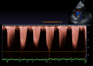
102. El Doppler.Nociones Básicas. Doppler Color.
107. Ecografía Pediátrica. Consideraciones.
108. Ecografía de Caderas neonatal
109. Ecografía de Abdomen Pediátrica.
113. Suprarrenales o Adrenales.
117. Estenosis hipertrófica de píloro.
121. SNC en Pediatría.Consideraciones.
122. Ecografía Transfontanelar. Cortes Coronales.
123. Ecografía Transfontanelar. Cortes Sagitales.
124 Ecografía Transfontanelar. Estudio Vascular básico.
125. Ecografía Transfontanelar,otros accesos.
126. Ecografía Transfontanelar. Patología básica.
128.SNC.Canal Medular.Patología básica.
130. Doppler Venoso Profundo MMSS. Consideraciones Generales.
132. Contraste Ecográfico. Consideraciones básicas.
133. El Contraste en Ecografía. El Nódulo hepático.
138. Ecocardiografía. Consideraciones generales
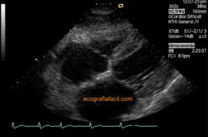
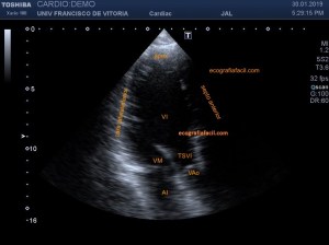
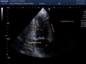
139. Ecocardiografía. Estudio Paraesternal Eje Largo.
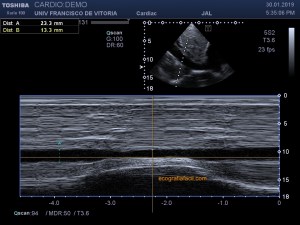
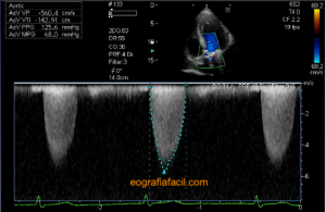
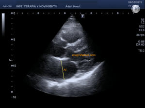
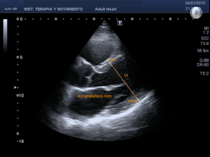
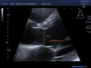
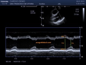
141. Mediciones de los planos paraesternales.
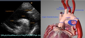
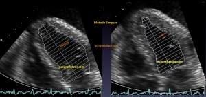
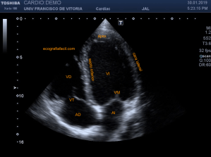
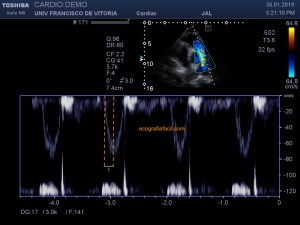
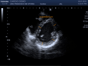
142. Ecocardiografía.Plano Apical 4 cámaras
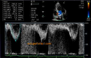
143. Ecocardiografía.Plano Apical 5 Cámaras.
144. Ecocardiografía.Plano Apical 2 Cámaras.
145. Ecocardiografía.Plano Apical 3 Cámaras.
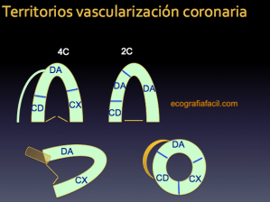
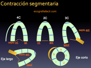
146. Ecocardiografía.Segmentación y territorios vasculares.
147. Ecocardiografía. Planos Subcostales.
148. Ecocardiografía. Planos Supraesternal y Paraesternal derecho.
149. Gracias, Ecocardiografía.
151. Denervación Muscular. Caso clínico.
155. Ecografía en Pediatría.Protocolos habituales,repaso.
159. Elastografía. Conceptos básicos.
160. La imagen ecográfica. Semiología y repaso.
162. Los Riñones, un abordaje diferente.
163. Artefactos de Electricidad.
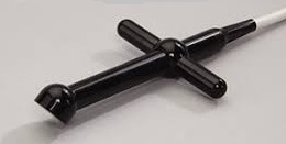
165. Dispositivos Subdérmicos.
168. Urotelioma en Divertículo vesical.
169. La tormenta de Nieve. Siliconomas.
171. Doppler: Tipos y usos en Tendinopatías.
174. Implante metastásico subcutáneo.
178. ¿Dilatación Renal o Quistes Renales?
180. Inserción Biceps, cabeza de Radio, acceso posterior.
182. La enfermedad de Osgood-Schlatter
183. Trombosis parcial de la vena Safena Interna.
184. Litiasis renales. Rx, TC y Ecografía.
185. Rx Portátil. Técnica del “arrastrón”.
186 Entesopatía y estudio de la inserción proximal del recto anterior del muslo.
187. Neuroma de Morton. Maniobra de movilización.
188. Cola de Páncreas. Técnica del vaso de agua.
189. Hiperplasia Nodular Focal.
190. Patología maligna del Testículo. Semiología habitual.
191. Rotura de Tendón Supraespinoso. Tipos y Semiología.
192. Divertículo esofágico de Killiam-Jamieson.
193. Edema y Absceso en ecografía. Semiología habitual.
195. Rotura de la placa plantar.
197. El Doppler y su evolución.
198. Psudoaneurisma renal con hematoma y angiomilipoma.
199. Nódulo de la hermana Mary Joseph.
201. Manejo de equipos y ajustes básicos en ecografía
202. Ectasia ductal y Papiloma intraductal.
205. Semiología y tumoración renal.
206. Calcificaciones distróficas + Síndrome de Haglund.
208. Clasificación Ti-Rads. Nódulos tiroideos.
210. Sartorio, rotura fibrilar
213. Hemorragia neonatal. Clasificación – Grados.
216. Calcificaciones migradas.
217. Calcificación inserción del tendón pectoral.
218. Protocolo básico Ecografía Doppler Renal.
222. Paraganglioma de cordón espermático.
225. Epitelioma calcificado de Malherbe o Pilomatrixoma.
229. Fractura cabeza de radio.
230. Tumor de Células Gigantes
231. Pseudoaneurisma de vaso superficial.
233. Artefactos que “emborronan” la imagen.
234. Quiste ovárico ¿Hemorrágico?
235. Candidiasis cerebral neonatal.
237. Neuropatía del Nervio Radial.
240. Curso de Ecografía para TSIDMN
241. Rotura del Extensor Largo del Pulgar. Tercer Compartimento.
242. La Vesícula, Adenomiomatosis y Gorro Frigio
244. Absceso Muscular por Staphilococo
245. INTERACCIÓN DEL HAZ DE US CON LA MATERIA.
246. Segunda Edición Del Curso de Ecografía para TSIDyMN NIVEL 1.
249. Atrofia grasa de los Rectos Abdominales.
250. Ecografía de Tórax, Líneas A y B.
251. Triple Patología Vesicular.
254. Muñeca de bebé. Enfermedad de De Quervain
256. Lipoma Intramuscular del Músculo Romboides.
257 El Síndrome del Cascanueces.
258. I Congreso Nacional de Ecografía para TSID. Octubre 2022.
259. Mastectomía bilateral. Lesión pectoral.
262. Quiste Hidatídico Calcificado.Clasificación de Gharbi.
266. Hemorragia Suprarrenal Neonatal Izquierda